AIS June 2019 Newsletter
Market Update
(all values as of 06.28.2024)

Stock Indices:

Dow Jones 39,118
S&P 500 5,460
Nasdaq 17,732

Bond Sector Yields:

2 Yr Treasury 4.71%
10 Yr Treasury 4.36%
10 Yr Municipal 2.86%
High Yield 7.58%

YTD Market Returns:

Dow Jones 3.79%
S&P 500 14.48%
Nasdaq 18.13%
MSCI-EAFE 3.51%
MSCI-Europe 3.72%
MSCI-Pacific 3.05%
MSCI-Emg Mkt 6.11%
 
US Agg Bond -0.71%
US Corp Bond -0.49%
US Gov’t Bond -0.68%

Commodity Prices:

Gold 2,336
Silver 29.43
Oil (WTI) 81.46

Currencies:

Dollar / Euro 1.06
Dollar / Pound 1.26
Yen / Dollar 160.56
Canadian /Dollar 0.73

Macro Overview

The ongoing trade dispute between the U.S. and China escalated in May as the U.S. signaled that it had not finalized a deal yet with China. The lack of a deal led to the U.S. announcing an increase in tariffs from 10 percent to 25 percent on $200 billion of Chinese imports.

The U.S. Department of Commerce began assessing Chinese imports arriving at U.S. ports with a 25% tariff at 12:01 AM on June 1st. The tariff increase affects a broad range of imported products, including modems, routers, furniture, and vacuum cleaners. Additional tariffs were also proposed by The Office of the United States Trade Representative on essentially all remaining imports from China, valued at about $300 billion.

The proposed tariff increases by the United States caused China to retaliate against the U.S. with its own tariff proposals on U.S. goods including alcohol, swimsuits, and liquefied natural gas (LNG). The Chinese government may apply additional tariffs to more impactful products including food, energy and aircraft products from the U.S.

The recent market downturn has primarily been due to the uncertainty of the trade disputes and the effects of tariffs on the U.S. and international economies. Analysts believe that the equity market pullback along with the pending trade disputes have raised the possibility of an interest rate cut by the Federal Reserve later this year.

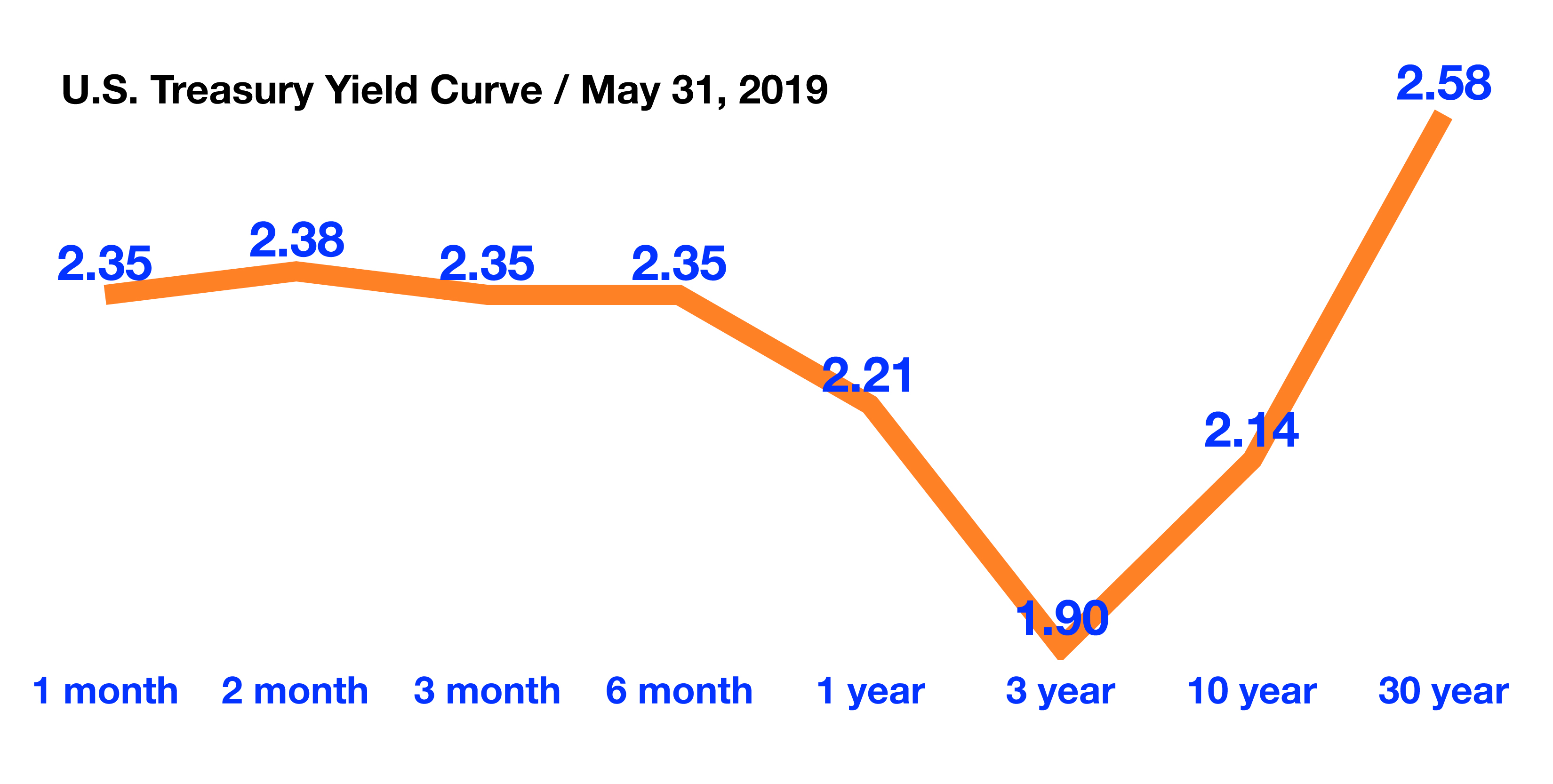
Longer term U.S. Treasury bond yields fell to their lowest levels since 2017. Combined pressures from the trade disputes to the pending Brexit turmoil in Europe has fostered increasing demand for U.S. Treasury bonds, which has resulted in higher bond prices.

The fixed income market is looking at the probability that economic weakness will lead to the Federal Reserve to actually cut interest rates sometime this year in order to bolster the U.S. economy. Many believe that the Fed needs to move quickly in order to shore up growth at the first sign of any economic contraction.

Mortgage rates fell below 4% for the first time since early last year helping to stabilize housing market activity. The average mortgage rate on a 30-year fixed conforming loan was 3.99% at the end of May, as tracked by Freddie Mac, the lowest since January 2018. Falling mortgage rates tend to entice buyers to sell their homes and trade up to larger homes with bigger mortgage balances, a boom for the housing market.

The most recent unemployment data revealed that unemployment unexpectedly fell to a 50 year low this past month to 3.6 percent, the lowest since 1969. Historically, a low unemployment rate tends to drive consumer confidence higher and act as a buffer during economic uncertainty.

Canada, Mexico, and the United States introduced legislation that would replace the North American Free Trade Agreement (NAFTA) and establish a new trade treaty among the three countries to be referred as the U.S.-Mexico-Canada Agreement (USMCA). Existing tariffs on steel and aluminum imports from Canada would be eradicated. Canada is the second largest foreign supplier of steel and aluminum to the United States.

Sources: Dept. of Commerce, Treasury Dept., Freddie Mac, IMF

 
$10.6 trillion worth of global debt is now in negative yielding territory

Rates Drop Rapidly Amid Inverted Yield Curve – Fixed Income Update

Markets tend to look at the yield curve in order to find clues as to what the expectations are about future economic growth and inflation. The yield curve is essentially the current yield on government Treasury bonds from 3-month maturities to 30-year maturities. At the end of May, the 1, 2, 3, 6 month and 1-year notes all yielded more than the benchmark 10-year bond. When shorter term bonds are yielding more than longer term bonds, it is known as an inversion or inverted yield curve.

Economically sensitive copper and oil prices fell in May, perhaps signaling weaker global growth activity. Such dynamics in the commodities market tends to push yields lower internationally. Some analysts believe that a continued escalation of trade disputes with countries in addition to China will crimp global economic growth and force the Federal Reserve to lower interest rates.

Total global debt as of the end of 2017 was $184 trillion, as monitored by the International Monetary Fund (IMF). Global bond yields fell in May with an estimated $10.6 trillion worth of debt now in negative yielding territory, the highest since 2016.

Some fixed income analysts are projecting lower yields later this year due to slowing economic expansion, continued demand for U.S. government debt, and an increasing probability that the Fed will eventually lower rates. (Sources: IMF, Treasury Dept., Federal Reserve)

Equities Give Up Early Gains – Equity Market Update

In stark contrast to the strong performance during the first four months of 2019, U.S. equities faltered in May as continued trade disputes hindered economic growth expectations. All sectors of the S&P 500 Index fell in May, with the exception of Real Estate. Technology and financial stocks experienced the brunt of the pullback in May.

May was the worst month since December 2018, when markets reacted to heightening trade fears and a possible rate hike by the Federal Reserve. Ironically, some analysts are expecting a reduction in rates by the Fed later this year in response to tariff reverberations and slowing economic global growth. A rate decrease by the Fed might lure equities higher as loan costs and capital remain inexpensive, thus buffering profit margins for U.S. companies.

Should a continued drop in rates persist, economists note that the U.S. dollar may weaken, thus boosting U.S. multi-national company earnings, which primarily operate internationally.

Global inflation expectations have eased considerably over the past month, prompting central banks in various countries to consider lowering rates, also known as growth stimulus efforts. (Sources: S&P, Bloomberg, Federal Reserve)

 
Yield Curve Steepening Trade Update

YIELD CURVE STEEPENING TRADE UPDATE

Last summer we issued a special report on a special type of corporate bond with a coupon that adjust based on the steepness of the yield curve.  The coupon is calculated using a formula which differs for each bond. As the yield curve steepens the coupon goes up and if it flattens the coupon adjust down.  As the yield curve flattened throughout most of last year the coupons were resetting lower each quarter until they finally hit zero last year.  Obviously, the prices fell precipitously as the coupons went to zero and these bonds were trading at in the $50 – $60 range – keep in mind these are investment grade corporate bonds that are issued by the largest financial institutions in the world (BofA, Citigroup, SocGen, etc.) and the quality of the underlying credit had not changed.  These bonds are generally marketed to retail investors at $100 and as one can imagine as the coupons fell and prices plummeted there was mass panic selling.   It was our thesis that the sell-off was overdone as the bonds were trading at significant spreads to the treasury curve assuming a zero coupon for life.  Bonds could be purchased at 4%+ yields assuming no coupon for the life of the bond which meant investors were getting an option for free.  The table below shows the current levels for the most commonly quoted curves:

The majority of yield curve steepener notes use the 2’s to 30’s or the 5’s to 30’s curves (#’s 15 and 20 in the table) and as you can see they are not only the widest curves but also both are currently the furthest outside their 1 year average. When we published our special report last year the 5-30 curve was 12bps and was -2.13 standard deviations its  historic average.  As you can see in the table above (second to last column on right) this has completely reversed and it is now +2.08 standard deviations its 1 year average.  At the time we issued the report we took a 10-15% allocation in client accounts and the bonds have since increased in value 10% -25% depending on the issuer, formula and maturity.  We are still holding our original position but are remaining cautious due to our negative view on credit spreads and the corporate bond market (discussed on the next page).


Credit spreads and the Corporate Bond Market

In May Jeffrey Gundlach (the new bond king), founder of Doubleline Capital gave an interview in which he said the corporate bond market could be heading for a collapse that would rival the sub-prime crisis of 2008.  And that while corporate bonds are not as over-valued as sub-prime mortgage debt was prior to the financial crisis, the corporate bond market dwarfs the sub-prime mortgage market and the overall exposure to investors could be the same.

If this sounds familiar to our regular readers it is because we have been echoing this thesis for over a year.  According to Gundlach, corporate bonds have been rich (expensive) by one standard deviation for most of the last 3 years and are now at an “outright sell” level.   He added that based on corporate leverage ratios, 38% of the corporate bond market should be rated junk.  The high-yield market is just as expensive as the investment grade market, Gundlach said, and spreads are totally inconsistent with corporate debt levels.  The chart below was from Jeffrey Gundlach’s DoubleLine Asset Allocation webcast for the month of November 2018:

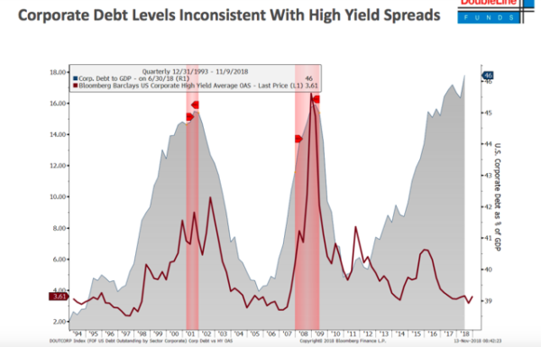
This chart clearly shows spreads (the risk premium investor receive for buying corporate bonds) is not only historically low but that given the massive amount of corporate debt spreads are reaching stratospheric levels which are not sustainable.  The small stock market sell-off in the last quarter of 2018 gave us a glimpse into how quickly liquidity can dry up and bond spreads can dramatically widen in a high volatility environment and that was not even a major event.  We have written extensively in previous newsletters and illustrated how quickly bond prices can spiral downward in a high volatility environment.  In 2008 it was sub-prime mortgage’s that sent the markets reeling, the next crisis will almost certainly be caused by this combination of massive corporate debt and historically tight spread levels.

Gundlach went on to echo another theme of ours, that most of global GDP growth has been based entirely on the huge explosion of global debt of all types – government, corporate and even mortgage and consumer debt.  We have consistently beat the drum that this global debt bubble is almost certain to implode – it simply is not possible to continue to print and borrow money at these rates without serious fallout.  Considering the flat/inverted yield curve corporate bond investors would be wise reduce risk by either lowering their allocation to the sector of shortening the duration of their holdings.


Retirement Planning - When to Take Social Security

Deciding When To Take Social Security – Retirement Planning

Deciding when to take Social Security benefits is one of the most important decisions one will make for retirement. You may either base the decision strictly on monetary benefits, or your decision may be more personally based.

The important question is when to start taking benefits, at age 62 or postponing benefits until age 66, or even later. The answer is different for everyone, as it depends on various factors such as health, lifestyle, and marital status. The amount of your monthly benefit depends on two variables, when you elect to start receiving them, and how much you’ve earned during your working years.

To determine how much you’ve earned, the Social Security Administration adds up the income subject to Social Security tax adjusted for inflation during your 35 highest-earning years. It then divides that total by 420, the number of months in 35 years. This figure arrives at your average indexed monthly earnings. The higher this is, the higher your benefits will be.

The Social Security Administration designs the benefit formula based on an average, so the same amount of lifetime benefits is calculated irrespective of when you begin receiving payments. The U.S. Government Accountability Office (GAO) explains this in a report on social security retirement saying “the Social Security benefit formula adjusts monthly payments so that someone living to average life expectancy should receive about the same amount of benefits over their lifetime regardless of which age they claim”.

When it comes to deciding as to what age to start taking benefit payments, various strategies and philosophies come into play. The calculated benefit amount per the Social Security Administration is known as the “full benefit”, in essence providing 100% of the calculated benefit due.

The caveat is that you need to be at least 66 years of age to take the full benefit amount. For workers retiring in 2014, the full retirement age is currently 66. However, if you elect to receive them earlier, then your monthly benefit is reduced for each month short of your 66th birthday. If you begin receiving them at age 62 for example, then your benefit will be reduced by 25%.  Conversely, if you wait until turning 70, then you’re entitled to delayed retirement credits, which increase your benefits by 8% for each year of deferment, capping out at a total of 32%.

So how do you determine the optimal age to take benefits and whether or not waiting may be worthwhile? A break-even analysis can be done, thus calculating how much more in benefits you may get, either by waiting for a higher benefit say age 70, or taking a lower benefit at a younger age such as 62.


CONTINUED ON NEXT PAGE

 
Retirement Planning - When to Take Social Security

Essentially, if you decide to wait, then you lose out on payments you could have been receiving since age 62. If you wait, yes the benefit payment will be higher, but you may end up receiving less overall benefit payments if you die sooner than expected.

This is when you need to consider your personal factors, since a break-even analysis tells you nothing about these relevant and important facts. Important personal factors to consider include health, family life expectancy, marital status, immediate financial needs, and quality of life.

For example, if you have health ailments and suffer from medical conditions that may prohibit you from enjoying a lasting quality of life, take the benefits at an earlier age.

If you’re married and about to become eligible for benefits, then perhaps one should take the benefit first, with the second postponing benefits until an older age. The postponement of the second would yield a higher payment when benefits would begin.

Regardless of what your factors might be, careful review of all of your options from a financial and personal viewpoint are prudent in order to arrive at the best decision for you.

Sources: Social Security Administration, GAO